Karpenter — monitoring: its metrics and creating a Grafana dashboard for Kubernetes WorkerNodes with examples of PromQL queries

We have an AWS Elastic Kubernetes Service cluster with Karpenter which is responsible for EC2 auto-scaling, see AWS: Getting started with Karpenter for autoscaling in EKS, and its installation with Helm.
In general, there are no problems with it so far, but in any case we need to monitor it. For its monitoring, Karpenter provides metrics out of the box that we can use in Grafana and Prometheus/VictoriaMetrics alerts.
So, what we will do today:
- add Karpenter metrics collection to Prometheus/VictoriaMetrics
- will see which metrics can be useful to us
- will create a Grafana Dashboard for WorkerNodes + Karpenter
In general, this post is more about Grafana than Karpenter, but the in Grafana graphs we will mainly use metrics from Karpenter.
We will also need to create alerts, but that’s for another time. Having an idea of the available Karpenter metrics and Prometheus queries for graphs in Grafana, you shouldn’t have any problems with alerts.
Let’s go.
Collecting Karpenter metrics with VictoriaMetrics VMAgent
Our VictoriaMetrics has its own chart, see VictoriaMetrics: deploying a Kubernetes monitoring stack.
To add a new target, update the values of this chart, and add the endpoint karpenter.karpenter.svc.cluster.local:8000:
...
  vmagent:
    enabled: true
    spec:
      replicaCount: 1
      inlineScrapeConfig: |
        - job_name: yace-exporter
          metrics_path: /metrics
          static_configs:
            - targets: ["yace-service:5000"]
        - job_name: github-exporter
          metrics_path: /
          static_configs:
            - targets: ["github-exporter-service:8000"]
        - job_name: karpenter
          metrics_path: /metrics
          static_configs:
            - targets: ["karpenter.karpenter.svc.cluster.local:8000"]
...
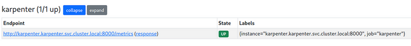
Deploy it and open a port to VMAgent to check the target:
$ kk port-forward svc/vmagent-vm-k8s-stack 8429
Check the targets:
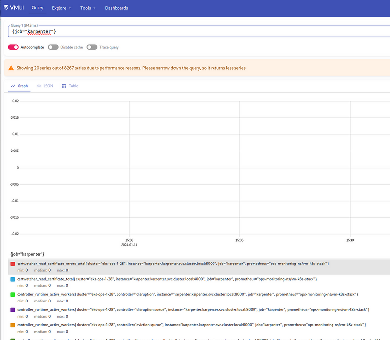
To check the metrics, open a port to VMSingle:
$ kk port-forward svc/vmsingle-vm-k8s-stack 8429
And look for data by the {job="karpenter"} query:
Useful Karpenter metrics
Now let’s see which metrics can be useful to us.
But before we get into the metrics, let’s talk about the basic concepts in Karpenter (besides the obvious ones like Node, NodeClaim, or Pod):
- controller : a Karpenter component that is responsible for a certain aspect of its operation, for example, the Pricing controller is responsible for checking the cost of instances, and the Disruption Controller is responsible for managing the process of changing the state of WorkerNodes
- reconciliation : the process when Karpenter reconciles the desired state and the current state, for example — when a Pod appears where there are no free resources on existing WorkerNodes, Karpenter will create a new Node on which the Pod can run, and its status will become Running — then the reconciliation process of the status of this Pod will be completed
- consistency : internal control process and ensuring compliance with the required parameters (for example, checking that the created WorkerNode has a disk of exactly 30 GB)
- disruption : the process of changing WorkerNodes in the cluster, for example, recreating a WorkerNode (to replace it with an instance with more CPU or Memory), or deleting an existing node that has no running Pods
- interruption : cases when an EC2 instance is stopped due to hardware errors, instance termination (when you do a Stop or Terminate instance), or in the case of Spot, when AWS “takes back” that instance (actually, its resources like CPU and Mem); these events go to a corresponding SQS, from where Karpenter receives them to launch a new instance to replace it
- provisioner : a component that analyzes the current needs of the cluster, such as requests for creating new Pods, determines which resources need to be created (WorkerNodes), and initiates the creation of new ones (in general, Provisioner has been replaced by NodePool, but some metrics for it remain)
Here I’ve collected only the metrics that I found most useful at the moment, but you should check out the Inspect Karpenter Metrics documentation for yourself and there’s a bit more detail in the Datadog documentation:
Controller :
-
controller_runtime_reconcile_errors_total: the number of errors when updating WorkerNodes (i.e. in the Disruption Controller when performing Expiration, Drift, Interruption and Consolidation operations) - it is useful to have a graph in Grafana or an alert -
controller_runtime_reconcile_total: the total number of such operations - it is useful to have an idea of Karpenter activity and possibly have an alert if it happens too often
Consistency :
-
karpenter_consistency_errors: looks like a useful metric, but I have it empty (at least for now)
Disruption :
-
karpenter_disruption_actions_performed_total: the total number of disruption actions (deleting/recreating WorkerNodes), the metric labels indicate a disruption method - it is useful to have an idea of Karpenter activity and possibly have an alert if it happens too often -
karpenter_disruption_eligible_nodes: the total number of WorkerNodes to perform disruption (deletion/recreation of WorkerNodes), the metric labels indicate disruption method -
karpenter_disruption_replacement_nodeclaim_failures_total: the total number of errors when creating new WorkerNodes to replace the old ones, the metric labels indicate disruption method
Interruption :
-
karpenter_interruption_actions_performed: the number of actions on EC2 Interruption notifications (from SQS) - maybe it makes sense, but I did not see this during the week of collecting metrics
Nodeclaims :
-
karpenter_nodeclaims_created: the total number of created NodeClaims with labels by reason of creation and the corresponding NodePool -
karpenter_nodeclaims_terminated: similarly, but for deleted NodeClaims
Provisioner :
-
karpenter_provisioner_scheduling_duration_seconds: it may make sense to monitor it, because if it grows but is too high, it may be a sign of problems; however, I havekarpenter_provisioner_scheduling_duration_seconds_buckethistogram unchanged
Nodepool :
-
karpenter_nodepool_limit: NodePool CPU/Memory limit set in its Provider (spec.limits) -
karpenter_nodepool_usage: NodePool resource utilization - CPU, Memory, Volumes, Pods
Nodes :
-
karpenter_nodes_allocatable: information on existing WorkerNodes - types, amount of CPU/Memory, Spot/On-Demand, Availability Zone, etc. - you can have a graph by the number of Spot/On-Demand instances
- can be used to obtain data on available CPU/memory resources —
sum(karpenter_nodes_allocatable) by (resource_type) -
karpenter_nodes_created: total number of Nodes created -
karpenter_nodes_terminated: total number of deleted Nodes -
karpenter_nodes_total_pod_limits: the total number of all Pod Limits (except DaemonSet) on each WorkerNode -
karpenter_nodes_total_pod_requests: total number Pod Requests (except DaemonSet) on every WorkerNode
Pods :
-
karpenter_pods_startup_time_seconds: the time from the creation of a Pod until to its transition to the Running state (the sum of all tax returns) -
karpenter_pods_state: is a pretty useful metric because it has the status of a Pod in the labels, on which Node it was launched on, its namespace, etc.
Cloudprovider :
-
karpenter_cloudprovider_errors_total: number of errors from AWS -
karpenter_cloudprovider_instance_type_price_estimate: the cost of instances by type - you can display the cost of cluster compute power on the dashboard
Creating Grafana dashboard
There is a ready-made dashboard for Grafana — Display all useful Karpenter metrics, but it is not informative at all. However, you can get some graphs and/or queries from it.
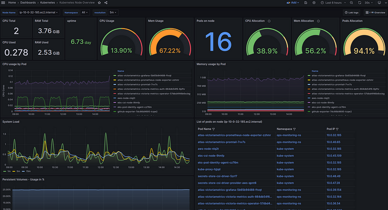
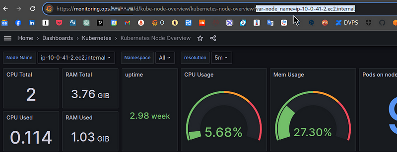
Now I have my own dashboard to check the status and resources for each individual WorkerNode:
In the graphs of this board, I have Data Links to dashboard with details on a specific Pod:
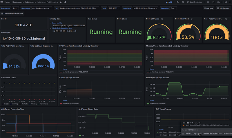
The ALB graphs below are built from logs in Loki.
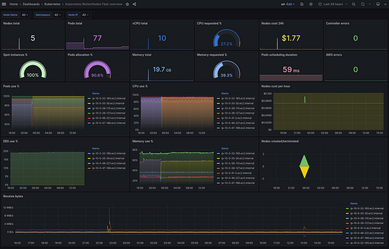
So what we’ll do is create a new board with all the WorkerNodes on it, and with the Data Links on the graphs of this board, we’ll link to the first dashboard.
Then there will be good navigation:
- a general board for all WorkerNodes with the ability to go to a dashboard with more detailed information on a specific Node
- on the board for a particular Node there will already be information about Pods on this Node, and data links to the board for a particular Pod
The dashboard planning
Let’s think about what we would like to see on the new board.
Filters/variables:
- be able to see all WorkerNodes together, or select one or more separately
- to be able to see resources by specific Namespaces or Applications (in my case, each service has its own namespace, so we will use them)
Next, information on Nodes:
- general information on nodes:
- number of Nodes
- number of Pods
- number of CPUs
- number of Mem
- spot vs on-demand ratio
- cost of all Nodes per day
- percentage of allocatable used:
- cpu — from Pods requested
- mem — from Pods requested
- Pods allocation
- real resources utilization — graphs by Nodes:
- CPU and Memory by Nodes
- number of Nodes — percentage of the maximum on the Node
- created-deleted Nodes (by Karpenter)
- Nodes cost
- percentage of EBS used
- network — in/our byes/sec
About Karpenter:
-
controller_runtime_reconcile_errors_total- total number of errors -
karpenter_provisioner_scheduling_duration_seconds- time of creation of Pods -
karpenter_cloudprovider_errors_total- total number of errors
Looks like a plan?
Let’s go.
Creating the dashboard
Create a new board and set the main parameters:
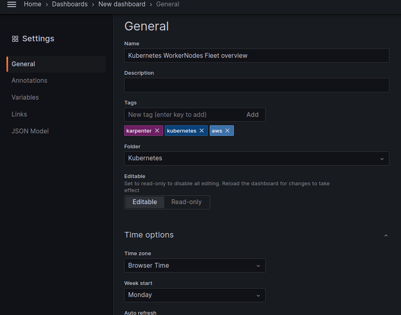
Grafana variables
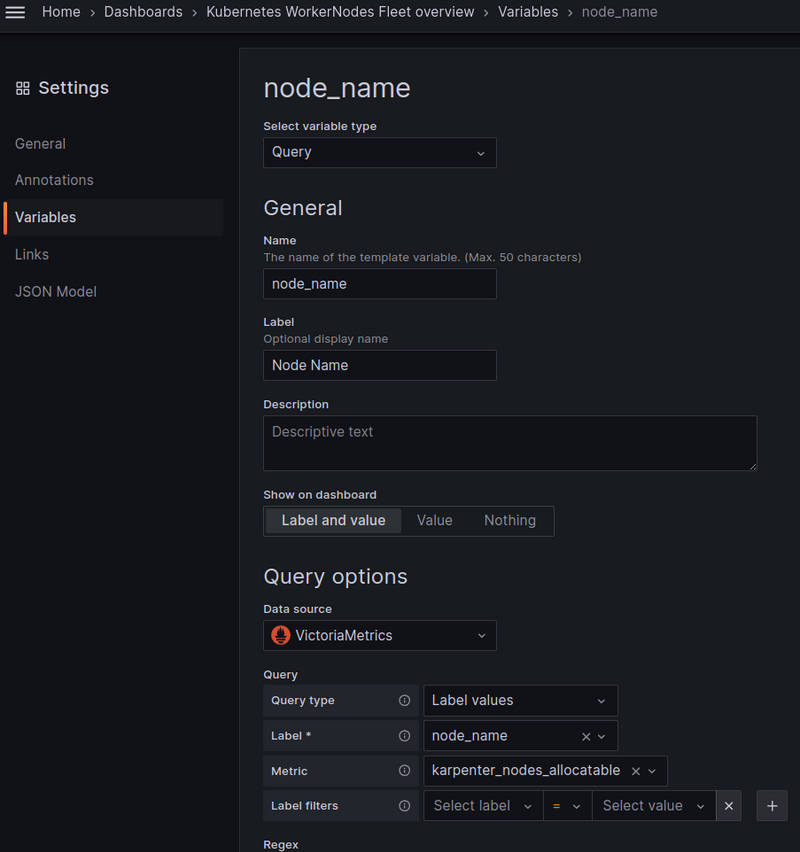
We need two variables — Nodes and Namespaces.
Nodes can be selected from the karpenter_nodes_allocatable, namespaces can be taken from the karpenter_pods_state.
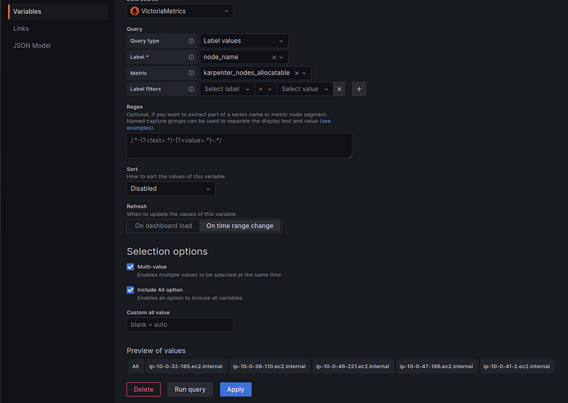
Create the first variable — node_name, include the ability to select All or Multi-value:
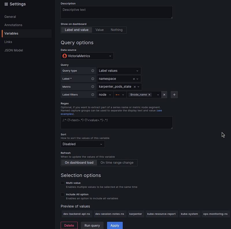
Create a second variable — $namespace.
To select namespaces only from the Nodes selected in the first filter, add the ability to filter by the $node_name that we created above and use a regular expression "=~" - if several Nodes are selected:
Let’s move on to the graphs.
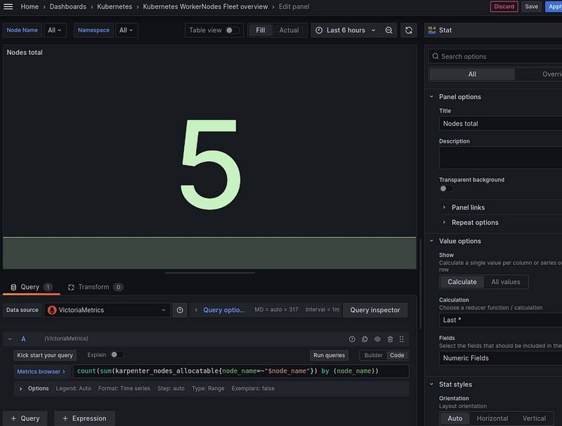
Number of WorkerNodes in the cluster
Query — use the node_name=~"$node_name" filter for the selected nodes:
count(sum(karpenter_nodes_allocatable{node_name=~"$node_name"}) by (node_name))
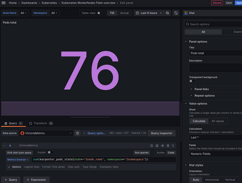
Number of Pods in the cluster
Query — here you can filter by both Nodes and Namespaces:
sum(karpenter_pods_state{node=~"$node_name", namespace=~"$namespace"})
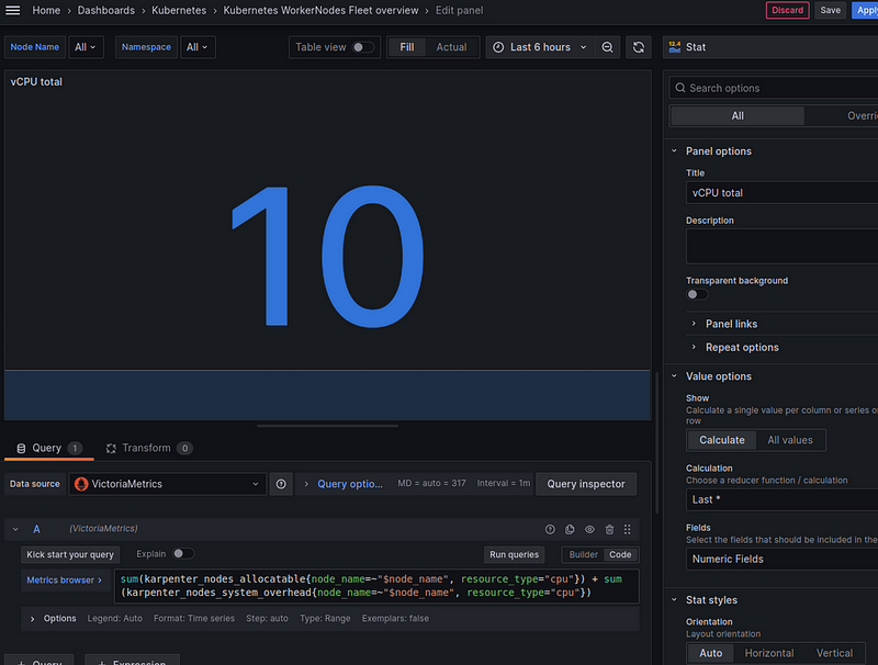
Number of CPU cores on all nodes
Some of the resources are occupied by the system or by DemonSets — they will not be taken into account in karpenter_nodes_allocatable. You can check with the query sum(karpenter_nodes_system_overhead{resource_type="cpu"}).
Therefore, we can output either the total amount — karpenter_nodes_allocatable{resourcetype="cpu"} + karpenter_nodes_system_overhead{resourcetype="cpu"}, or only the amount actually available for our workloads - karpenter_nodes_allocatable{resourcetype="cpu"}.
Since we want to see the total number here, let’s use the sum:
sum(karpenter_nodes_allocatable{node_name=~"$node_name", resource_type="cpu"}) + sum(karpenter_nodes_system_overhead{node_name=~"$node_name", resource_type="cpu"})
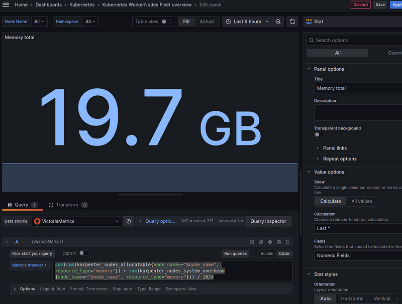
Total available Memory capacity
JFYI:
- SI standard: 1000 bytes in a kilobyte.
- IEC standard: 1024 bytes in a kibibyte
But let’s just make / 1024 ourselves and use Kilobytes:
sum(sum(karpenter_nodes_allocatable{node_name=~"$node_name", resource_type="memory"}) + sum(karpenter_nodes_system_overhead{node_name=~"$node_name", resource_type="memory"})) / 1024
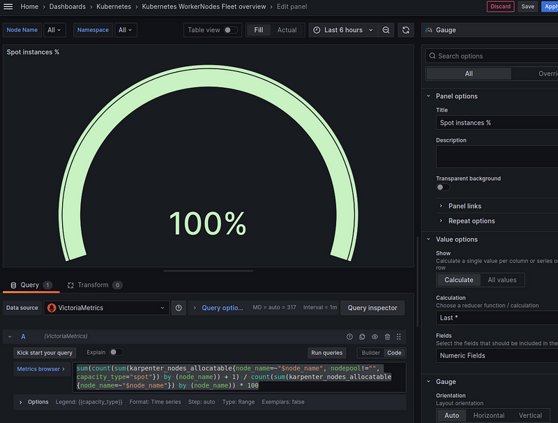
Spot instances — % of the total number of Nodes
In addition to the Nodes created by Karpenter itself, I have a dedicated “default” Node that is created when the cluster is created — for all controllers. It’s also a Spot (for now), so let’s count it as well.
The formula will be as follows:
spot nodes percent = all spot instances from karpenter + 1 default / total number of nodes
The query itself:
sum(count(sum(karpenter_nodes_allocatable{node_name=~"$node_name", nodepool!="", capacity_type="spot"}) by (node_name)) + 1) / count(sum(karpenter_nodes_allocatable{node_name=~"$node_name"}) by (node_name)) * 100
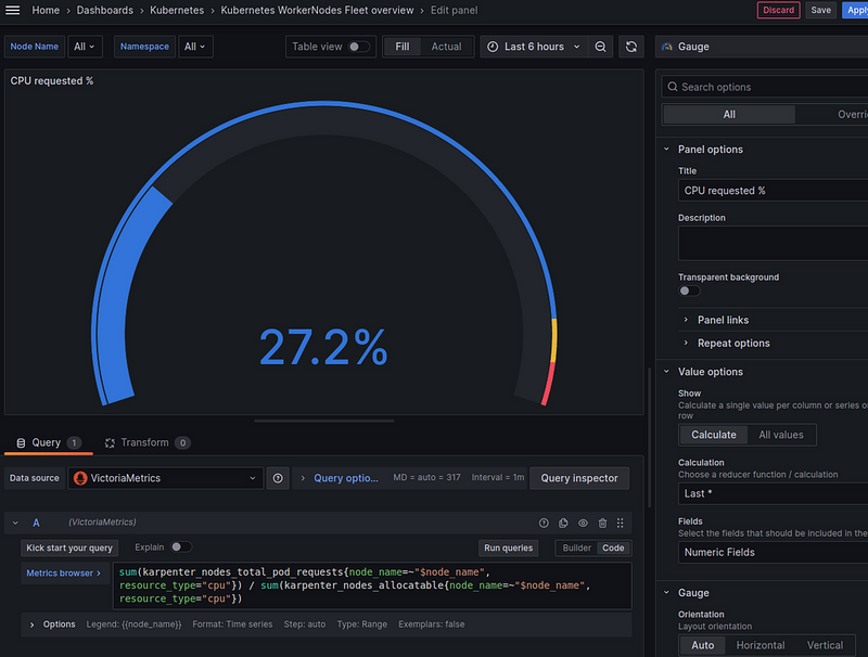
CPU requested — % of total allocatable
We take the query from the default Karpenter board and tweak it a bit to fit our filters:
sum(karpenter_nodes_total_pod_requests{node_name=~"$node_name", resource_type="cpu"}) / sum(karpenter_nodes_allocatable{node_name=~"$node_name", resource_type="cpu"})
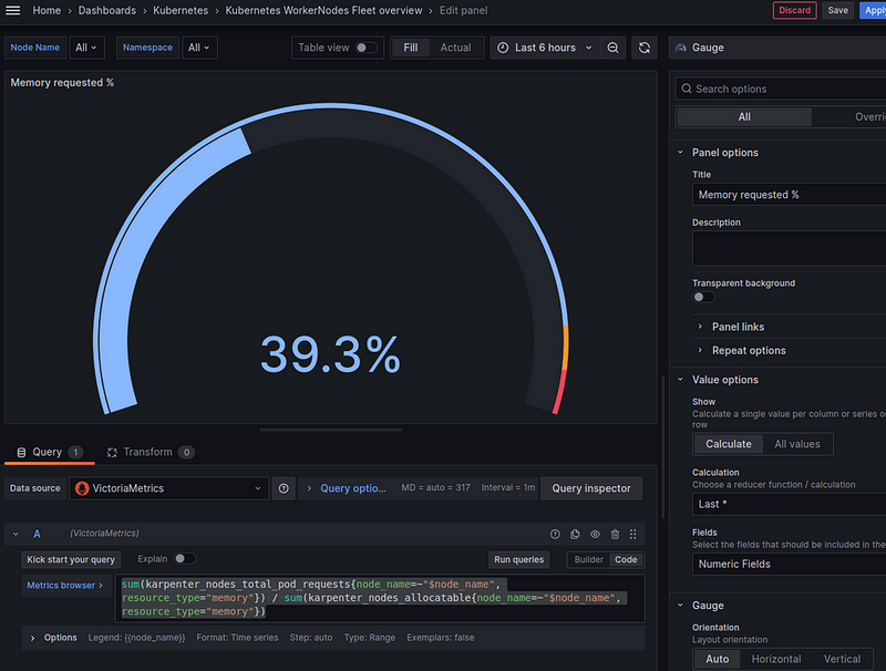
Memory requested — % of the total allocatable
Similarly:
sum(karpenter_nodes_total_pod_requests{node_name=~"$node_name", resource_type="memory"}) / sum(karpenter_nodes_allocatable{node_name=~"$node_name", resource_type="memory"})
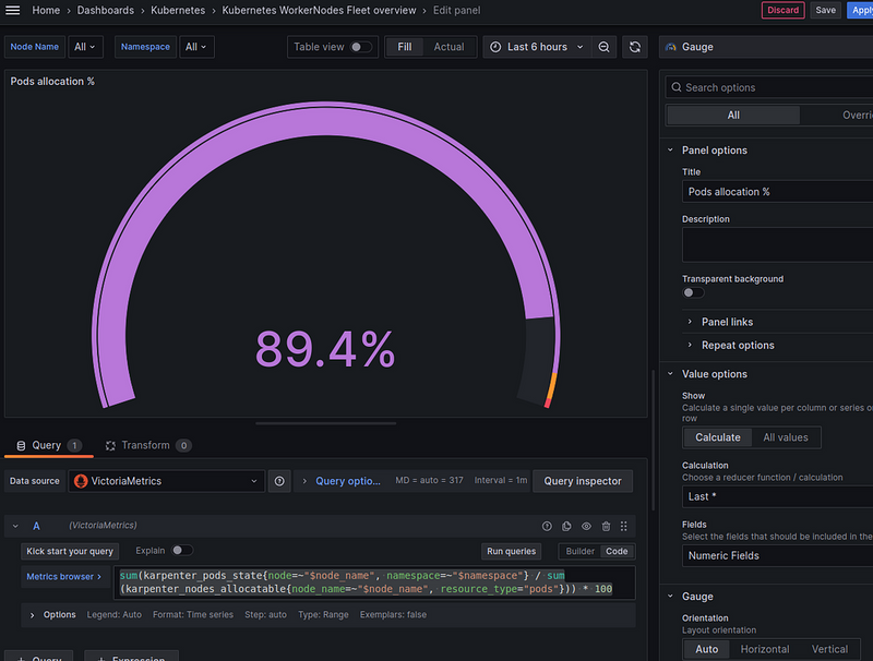
Pods allocation — % of the total allocatable
How many Pods do we have from the total capacity:
sum(karpenter_pods_state{node=~"$node_name", namespace=~"$namespace"} / sum(karpenter_nodes_allocatable{node_name=~"$node_name", resource_type="pods"})) * 100
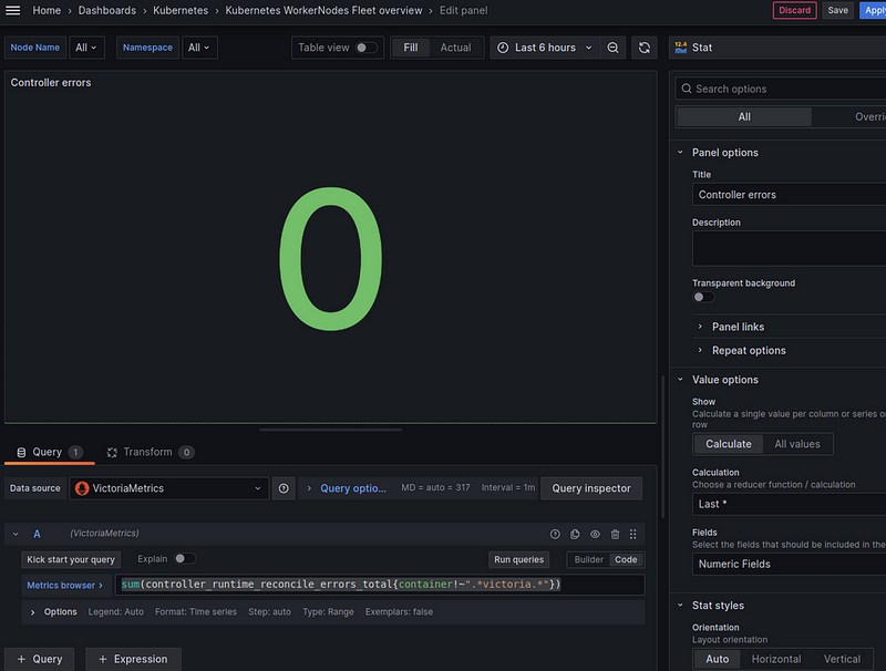
Controller errors
The controller_runtime_reconcile_errors_total metric includes controllers from VictoriaMetrcis, so we exclude them with {container!~".*victoria.*"}:
sum(controller_runtime_reconcile_errors_total{container!~".*victoria.*"})
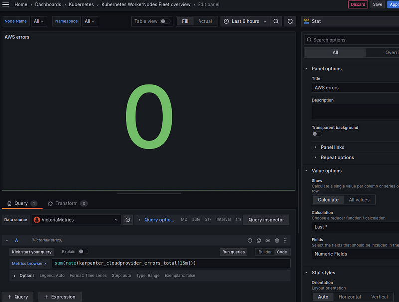
Cloudprovider errors
Count as a rate per second:
sum(rate(karpenter_cloudprovider_errors_total[15m]))
Nodes cost 24h — the cost of all Nodes per day
But here it turned out to be very interesting.
First of all, AWS has default billing metrics from CloudWatch, but our project uses AWS credits and these metrics are empty.
So let’s use Karpenter’s metrics — karpenter_cloudprovider_instance_type_price_estimate.
To display the cost of servers, we need to select each type of instance that is used and then calculate the total cost for each type and their number.
What do we have:
- the “default” Node: with Spot type, but not created by Karpenter — we can ignore it
- nodes created by Karpenter: can be either spot or on-demand, and can be of different types (
t3.medium,c5.large, etc.)
First, we need to get the number of nodes for each type:
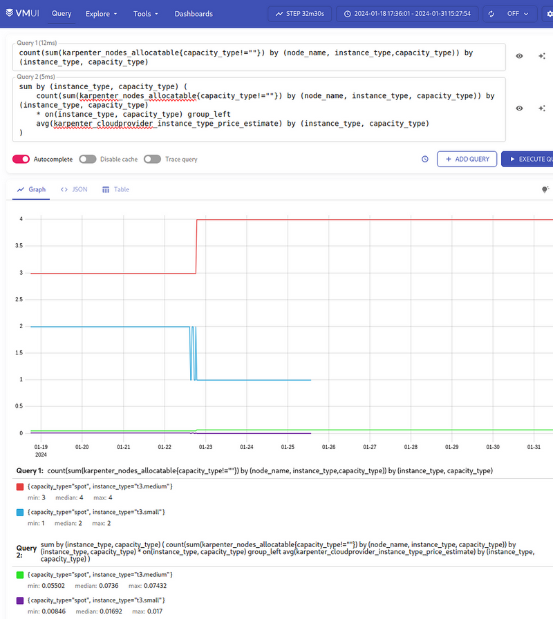
count(sum(karpenter_nodes_allocatable) by (node_name, instance_type,capacity_type)) by (instance_type, capacity_type)
We get 4 spots, and one instance without the capacity_type label, because it is from the default Node Group:
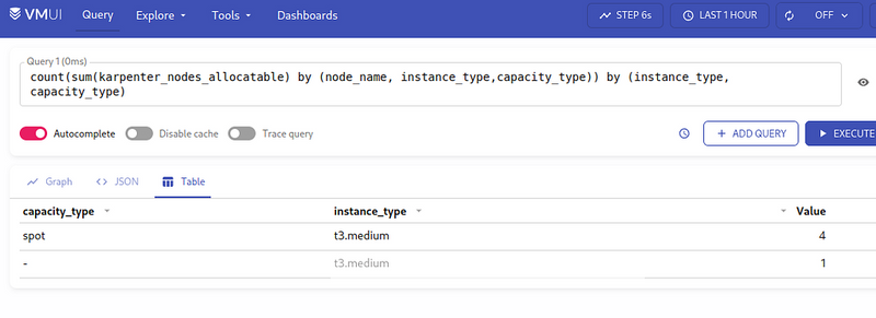
We can exclude it from {capacity_type!=""} - we have one, without autoscaling, we can ignore it, because it is only for the CriticalAddons.
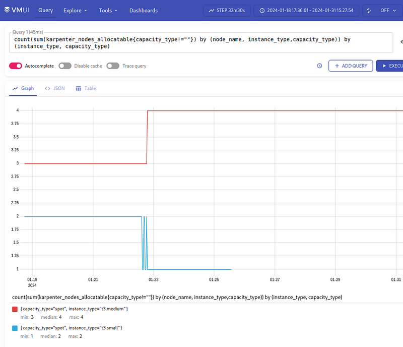
For a better picture, let’s take a longer period of time, because there was also t3.small:
Next, we have the karpenter_cloudprovider_instance_type_price_estimate metric, using which we need to calculate the cost of all instances for each instance_type and capacity_type.
The request will look like this (thanks to ChatGPT):
sum by (instance_type, capacity_type) (
    count(sum(karpenter_nodes_allocatable) by (node_name, instance_type, capacity_type)) by (instance_type, capacity_type)
    * on(instance_type, capacity_type) group_left
    avg(karpenter_cloudprovider_instance_type_price_estimate) by (instance_type, capacity_type)
)
Here:
- the “inner” query
sum(karpenter_nodes_allocatable) by (node_name, instance_type, capacity_type): calculates the sum of all CPUs, memory, etc. for each combination of thenode_name,instance_type,capacity_type - the “outer”
count(...) by (instance_type, capacity_type): the result of the previous query is counted with count to get the number of each combination - we get the number of WorkerNodes of eachinstance_typeandcapacity_type - second query —
avg(karpenter_cloudprovider_instance_type_price_estimate) by (instance_type, capacity_type): returns us the average price for eachinstance_typeandcapacity_type - using
* on(instance_type, capacity_type): multiply the number of nodes from query number 2 (count(...)) by the result from query number 3 (avg(...)) for the matching combinations of metricsinstance_typeandcapacity_type - and the very first “outer” query
sum by (instance_type, capacity_type) (...): returns the sum for each combination
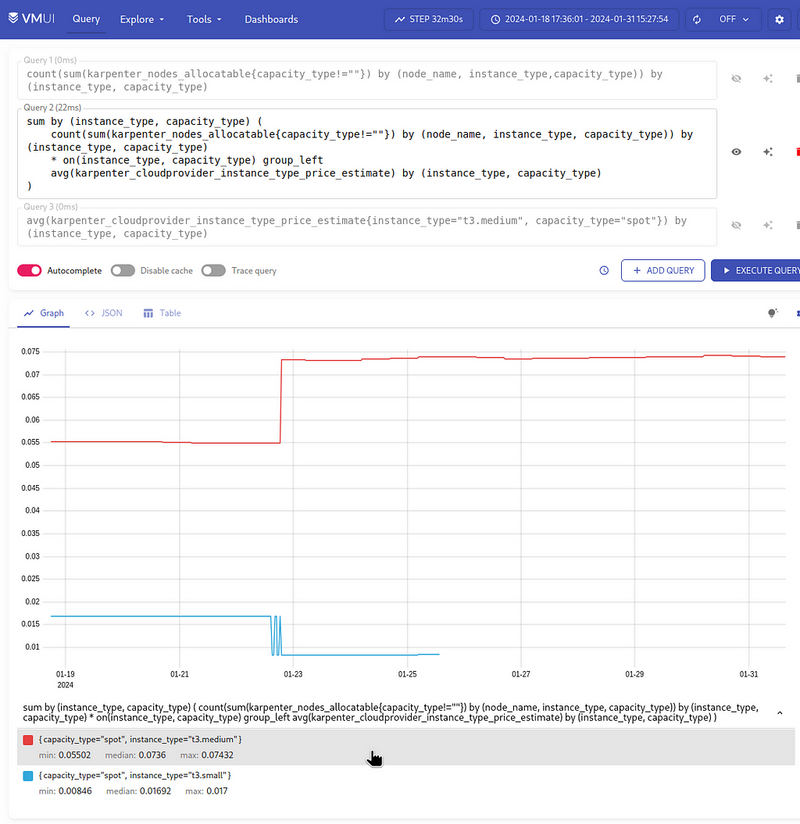
As a result, we have the following graph:
So, what do we have here?
- 4
t3.mediumand 2t3.smallinstances - the total cost of all
t3.mediumper hour is 0.074, allt3.small- 0.017
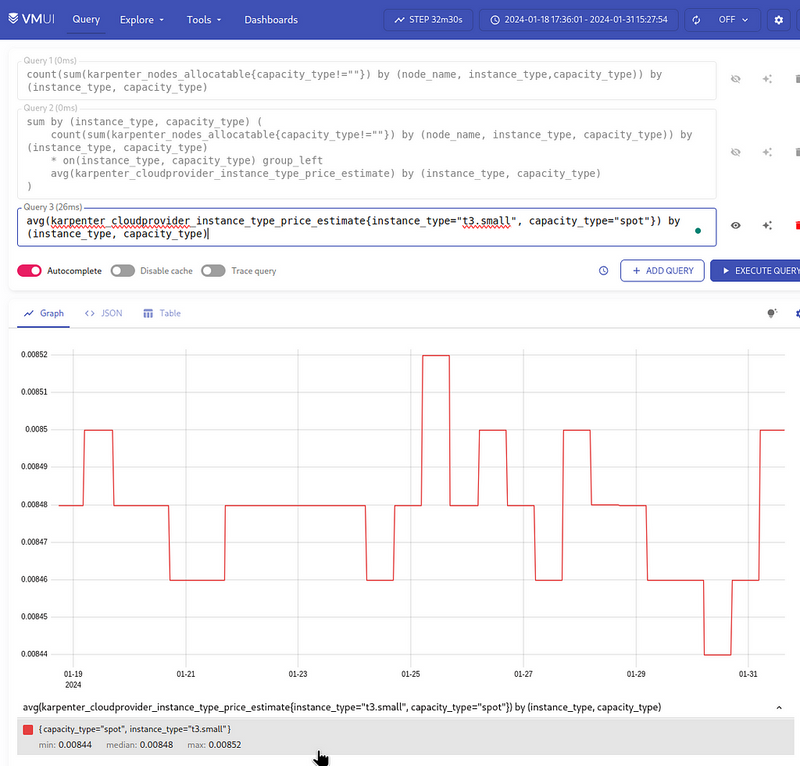
To check, let’s calculate it manually.
First, by the t3.small:
{instance_type="t3.small", capacity_type="spot"}
It turns out to be 0.008:
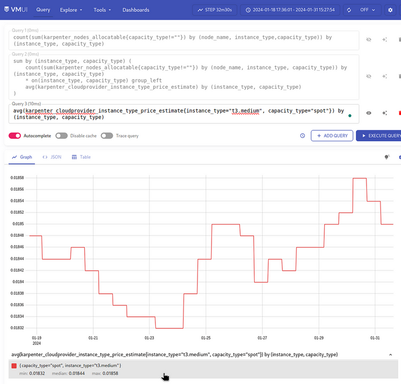
And by the t3.medium:
{instance_type="t3.medium", capacity_type="spot"}
This turns out to be 0.018:
So:
- 4 instances of
t3.mediumat 0.018 == 0.072 USD/hour - 2 instances of
t3.smallat 0.008 == 0.016 USD/hour
Everything looks correct.
All that’s left is to put it all together and display the total cost of all servers for 24 hours — use avg() and multiply the result by 24 hours:
avg(
  sum by (instance_type, capacity_type) (
    count(sum(karpenter_nodes_allocatable{capacity_type!=""}) by (node_name, instance_type, capacity_type)) by (instance_type, capacity_type)
    * on(instance_type, capacity_type) group_left
    avg(karpenter_cloudprovider_instance_type_price_estimate) by (instance_type, capacity_type)
  )
) * 24
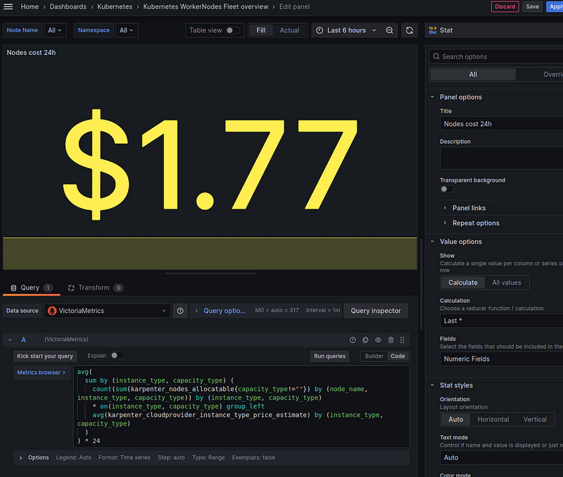
And as a result, everything looks like this:

Let’s move on to the graphs.
CPU % use by Node
Here, we will use the default metrics from Node Exporter — node_cpu_seconds_total, but they have instance labels in the form instance="10.0.32.185:9100", and not node_name or node as in Karpenter metrics (karpenter_pods_state{node="ip-10-0-46-221.ec2.internal"}).
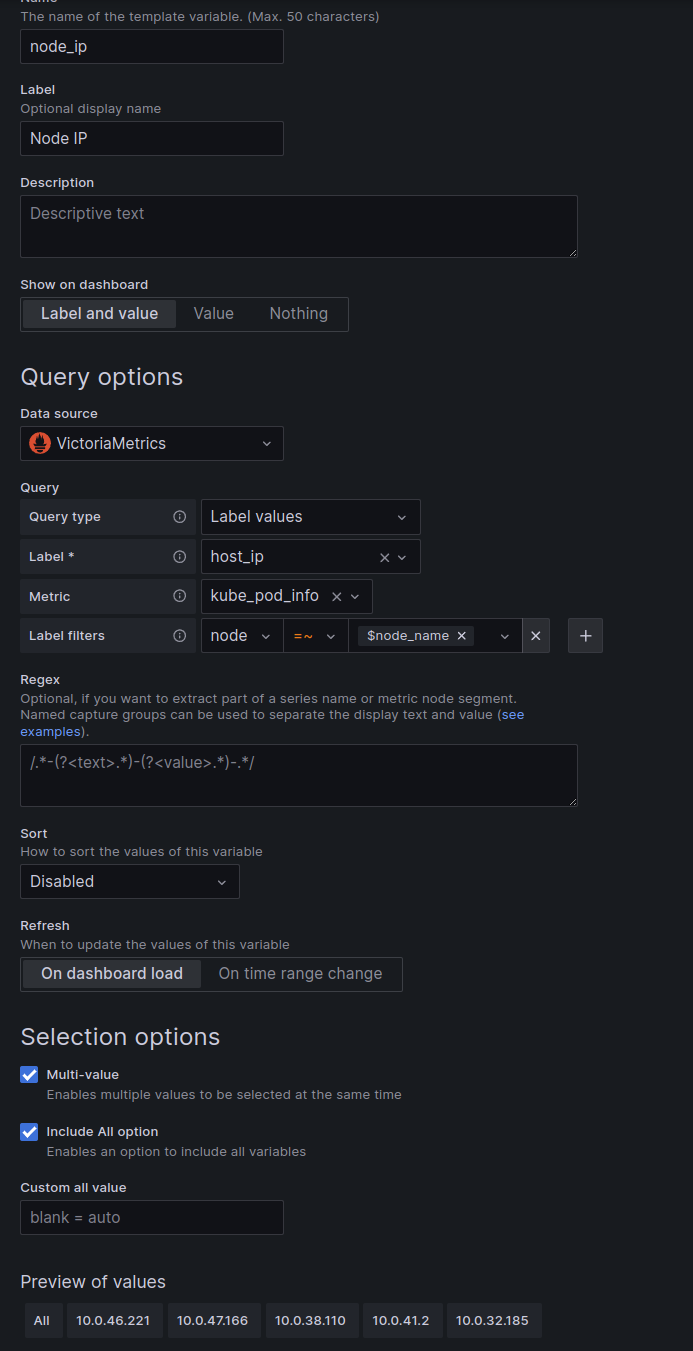
So to apply node_cpu_seconds_total with our variable $node_name we can add a new variable node_ip, which will be formed from the metric kube_pod_info with a filter by the label node, where we use our old variable node_name - to select Pods only from the Nodes selected in the filters.
Add a new variable, and for now, let to be the “Show on dashboard” enabled, for testing:
Now we can create a graph with a query:
100 * avg(1 - rate(node_cpu_seconds_total{instance=~"$node_ip:9100", mode="idle"}[5m])) by (instance)
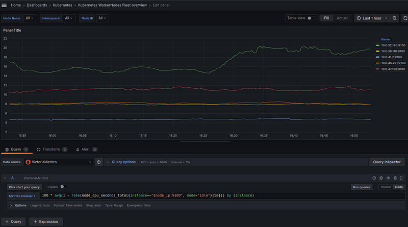
But in this case, the instance will return the results as "10.0.38.127:9100" - but we are using "ip-10-0-38-127.ec2.internal" everywhere. Also, we won't be able to add data links because the second panel uses the format the same format - ip-10-0-38-127.ec2.internal.
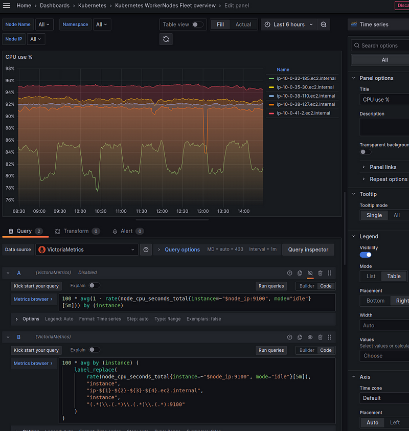
So we can use the label_replace() function and rewrite the request like this:
100 * avg by (instance) (
    label_replace(
        rate(node_cpu_seconds_total{instance=~"$node_ip:9100", mode="idle"}[5m]),
        "instance",
        "ip-${1}-${2}-${3}-${4}.ec2.internal",
        "instance",
        "(.*)\\.(.*)\\.(.*)\\.(.*):9100"
    )
)
Here, label_replace gets 4 aggregates:
- first — the metric on which we will perform the transformation (result
rate(node_cpu_seconds_total)) - the second is the label we will be transforming —
instance - third — a new value format for labels —
"ip-${1}-${2}-${3}-${4}.ec2.internal" - the fourth is the name of the label from which we will keep the data using regex
And lastly, we describe the regex “(.\*)\\.(.\*)\\.(.\*)\\.(.\*):9100", which should be used to get each octet from IPs like 10.0.38.127, and then write each result in the ${1}-${2}-${3}-${4} regex groups.
Now we have a graph like this:
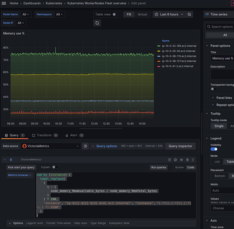
Memory used by Node
Everything is the same here:
sum by (instance) (
  label_replace(
    (
      1 - (
        node_memory_MemAvailable_bytes / node_memory_MemTotal_bytes
      )
    ) * 100,
    "instance", "ip-${1}-${2}-${3}-${4}.ec2.internal", "instance", "(.*)\\.(.*)\\.(.*)\\.(.*):9100"
  )
)
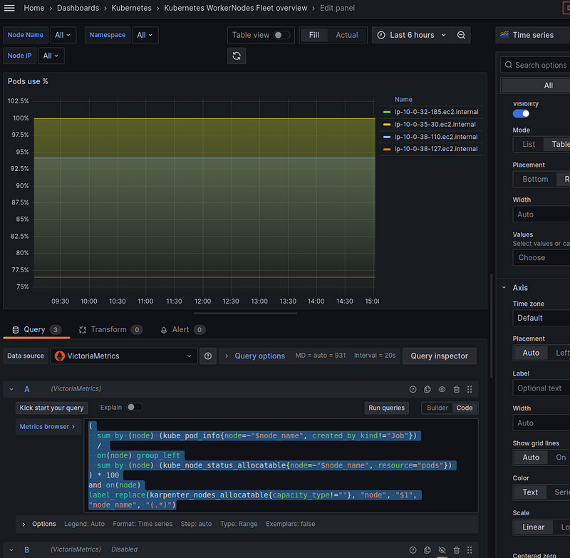
Pods use % by Node
Here we need to query between two metrics — karpenter_pods_state and karpenter_nodes_allocatable:
(
  sum by (node) (kube_pod_info{node=~"$node_name", created_by_kind!="Job"})
  /
  sum by (node) (kube_node_status_allocatable{node=~"$node_name", resource="pods"})
) * 100
Or we can exclude our default Node “ip-10–0–41–2.ec2.internal” and display only the Nodes of Karpenter itself by adding a selection by karpenter_nodes_allocatable{capacity_type!=""} - because we are more interested in how busy the Nodes created by Karpenter itself for our applications.
But for this, we need the karpenter_nodes_allocatable metric, where we can check for the presence of the capacity_type label - capacity_type!="".
However, karpenter_nodes_allocatable has a label node_name and not node as in the previous two, so we can add label_replace again and make this request:
(
  sum by (node) (kube_pod_info{node=~"$node_name", created_by_kind!="Job"})
  /
  on(node) group_left
  sum by (node) (kube_node_status_allocatable{node=~"$node_name", resource="pods"})
) * 100
and on(node)
label_replace(karpenter_nodes_allocatable{capacity_type!=""}, "node", "$1", "node_name", "(.*)")
Here, in the and on(node), we use the node label in the query results on the left (sum by()) and in the result on the right to select only those Nodes from the list of Nodes in karpenter_nodes_allocatable{capacity_type!=""} (that is, all Nodes except our "default" one) to select only those that are in the results of the first query:
EBS use % by Node
It’s easier here:
sum(kubelet_volume_stats_used_bytes{instance=~"$node_name", namespace=~"$namespace"}) by (instance)
/
sum(kubelet_volume_stats_capacity_bytes{instance=~"$node_name", namespace=~"$namespace"}) by (instance)
* 100
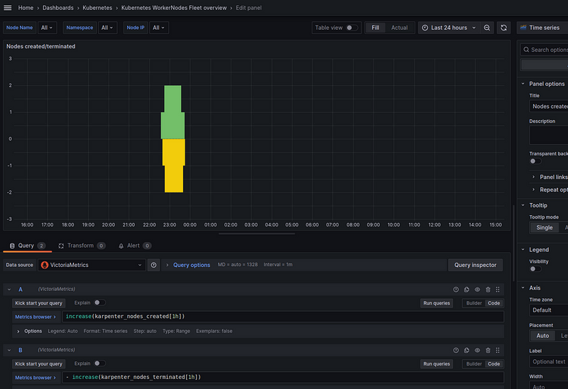
Nodes created/terminated by Karpenter
To display autoscaling activity, add a graph with two queries:
increase(karpenter_nodes_created[1h])
And:
- increase(karpenter_nodes_terminated[1h])
Here, in the increase() function, we check how much the value has changed in an hour:
And to get rid of these “steps”, we can additionally wrap the result in the avg_over_time() function:
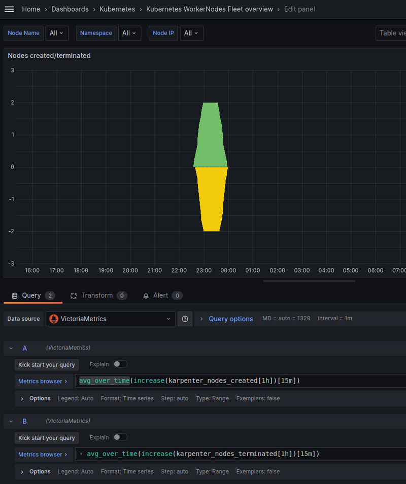
Grafana dashboard: the final result
And everything together now looks like this:
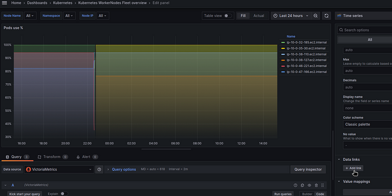
Adding Data links
The last step is to add Data Links to the panels: we need to add a link to another dashboard, for a specific node.
This dashboard has the following URL: https://monitoring.ops.example.co/d/kube-node-overview/kubernetes-node-overview?var-node_name=ip-10-0-41-2.ec2.internal.
Where var-node_name=ip-10-0-41-2.ec2.internal specifies the name of a Node on which the data should be displayed:
So open the panel and find Data links:
Set the name and URL — you can get a list of all fields by pressing Ctrl+Space:
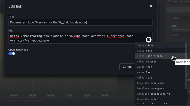
The __field will take values from the labels.node from the query result in the panel:
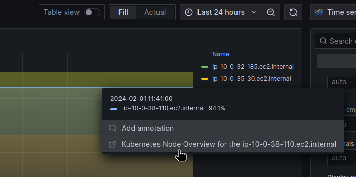
And will generate a link in the form “https://monitoring.ops.example.co/d/kube-node-overview/kubernetes-node-overview?var-node_name=ip-10-0-38-110.ec2.internal".
Originally published at RTFM: Linux, DevOps, and system administration.

Top comments (1)
This tool is handy for keeping an eye on your worker nodes in Kubernetes. It gives you a clear view of what’s happening with easy-to-read graphs in Grafana. It’s really helpful for making sure your system runs smoothly!